Introduction to MATLAB Tutorial Part 2: Worked Example

In part 1 of this tutorial, we covered basic concepts and syntax you need to use and write MATLAB code. In this part, we will put these tools to work to complete a simple data analysis task.

Task Definition
Preparation
Pseudocode
Define paramaters
Reading in data
Running scripts
Lake levels
Adding the main loop
Compute area and volume
Plotting the results
Convert script to a function

Task Definition

Write a program that reads gridded lake depth data from a text file and computes lake volume and area as functions of lake level. Include an option to plot the results. Use scripts or functions to make the analysis easily repeatable and reusable.

Input: Gridded water depth (bathymetry) for the Quabbin Resevoir in Central Massachussets. The the data are provided as comma separated values (a csv file) arranged from N-to-S in rows, and E-to-W in columns at 20 m spacing. The data are derived from bathymetric contours provided by the Massachusetts Dept. of Conservation & Recreation, available here.

Output: Resevoir volume and area as as function of lake level, optionally reported as a plot.

Preparation

Copy the bathymetry data file quabbin.csv to your working directory. You can do this from within MATLAB or using your system's file browser.

Create a new script and open up the Matlab Editor, either by clicking the New Script button on the upper right of the GUI, or typing

edit analyze.m

The name of the script is arbitary, but must have the .m extension.

Pseudocode

To start, think through the steps needed to accomplish the task. It is good practice to write out a rough outline of these, often called pseudocode.

I find it useful to frame up the new program by writing the pseudocode as comments, then to write the program by fleshing out this "skeleton". Comments are statements begining with % that are ignored by the MATLAB interpreter. They are for your eyes only and an essential tool for keeping track of what your code does (or intends to do).

% Script. Read gridded lake bathymetry data from a csv file and compute lake
% area and volume as a function of lake level.

% define parameters

% read in data

% get lake levels

% create output variables

% populate output variables

% loop: from maximum depth to empty
    % reduce level
    % compute area
    % compute volume
% loop: end

% plot, if enabled

Define paramaters

Since we are using a script, we need to define the input data explictly at the start of the script. We will need four peices of information: the data file name, the grid spacing, and the number of levels at which to compute area and volume. Like so:

% Script. Read gridded lake bathymetry data from a csv file and compute lake
% area and volume as a function of lake level.

% define parameters
file = 'data/quabbin.csv';
dx = 20; % m
dy = 20; % m
num_level = 10;

% read in data

% get lake levels

% create output variables

% populate output variables

% loop: from maximum depth to empty
    % reduce level
    % compute area
    % compute volume
% loop: end

% plot, if enabled

Reading in data

Before we try to read it in, it is a good idea to take a preliminary look at our dataset. You can do this with...

A text editor. The data are simply numbers separated by commas. * A spreadsheet program (e.g. MS Excel, LibreOffice Calc, etc). These programs know to read and display this data as an array.

The data are all positive or zero, which fits with our expectation. Since the data pass the smell test, we can move on to step one: read the dataset into a MATLAB variable.

We know what our data looks like (comma-separated values), and it seems likely that MATLAB has a tool to read in such a common data type. One way to check is to search the documentation. Type read csv into the search documentation toolbar. MATLAB suggests using the built-in function csvread. If we have a closer look at the documentation, MATLAB also tells us which input and output arguments this function has.

MATLAB needs to be able to see the data file to read it. MATLAB is aware of files in the current working directory and those explictly defined in the MATLAB path. Make sure that your current directory includes both your script analyze.m and the data file quabbin.csv.

Looking over the documentation shows us that we can load the data as follows:

depth = csvread('data/quabbin.csv');

This runs fine, and the new depth variable makes sense, it is a 2D matrix of dimension 1368x712. It is also probably a good idea to make a quick and dirty plot of the data. This prevents against the age old "garbage-in garbage-out" problem. Recall from part 1 that we can use the imagesc function to make 2D plots:

imagesc(depth)
colorbar

Adding the read command to the script gives:

% Script. Read gridded lake bathymetry data from a csv file and compute lake
% area and volume as a function of lake level.

% define parameters
file = 'data/quabbin.csv';
dx = 20; % m
dy = 20; % m
num_level = 10;

% read in data
depth = csvread(file);

% get lake levels

% create output variables

% populate output variables

% loop: from maximum depth to empty
    % reduce level
    % compute area
    % compute volume
% loop: end

% plot, if enabled

Running scripts

You run this (and any) script by typing its name at the command line, without the .m exentsion. MATLAB will search the current directory (and the MATLAB path) for a file with that name, and try to run it. To run our script, simple type analyze at the command line.

Note that the variables created in the script are now present in our workspace. This is important to remember: scripts share your workspace. They can see and alter variables in the current workspace. This can be useful (e.g. debugging, data exploration) and it can be dangerous (accidental overwrites, unexpected interactions between script and workspace). Just be aware!

Lake levels

To compute the volume and area at many lake levels, we will need to first create a vector of lake levels. Let's make these levels relative to the current (full) level - so a negative level corresponds to a less-than-full lake. Our level should go from full to empty. Here is one way to compute these levels.

% Script. Read gridded lake bathymetry data from a csv file and compute lake
% area and volume as a function of lake level.

% define parameters
file = 'data/quabbin.csv';
dx = 20; % m
dy = 20; % m
num_level = 10;

% read in data
depth = csvread(file);

% get lake levels
level_min = -max(max(depth));
level_step = level_min/(num_level-1);
level = 0:level_step:level_min;

% create output variables

% populate output variables

% loop: from maximum depth to empty
    % reduce level
    % compute area
    % compute volume
% loop: end

% plot, if enabled

Adding the main loop

We will want to compute area and volume for each value of level. To do this, we need to create empty (zero) vectors for the output data, and then create a loop that will populate each element of this variables.

For now, we leave the computations out and just assign dummy values to the outputs.

% Script. Read gridded lake bathymetry data from a csv file and compute lake
% area and volume as a function of lake level.

% define parameters
file = 'data/quabbin.csv';
dx = 20; % m
dy = 20; % m
num_level = 10;

% read in data
depth = csvread(file);

% get lake levels
level_min = -max(max(depth));
level_step = level_min/(num_level-1);
level = 0:level_step:level_min;

% create output variables
area = zeros(1, num_level);
vol = zeros(1, num_level);

% populate output variables
for i = 1:num_level

    % reduce level

    % compute area
    area(i) = 1;

    % compute volume
    vol(i) = 1;
end

% plot, if enabled

Compute area and volume

The next step is to compute the area and volume of the resevoir from the depth grid for each level.

Looking at the data, we can see that many of the datapoints in our matrix have a depth of zero, and thus lie outside of the resevoir. We must take care to exclude these points from our analyses.

To compute area, we wish to count all of the points within the resevoir, and multiply this by the area of each "pixel". We can identify points within the resevoir using a conditional test, take the sum of all elements of this matrix to count the points, and finally multiply be the cell dimesions to get the area in m^2

To compute volume, we can sum the depths of all the "wet" cells, and then multiply by the grid spacing.

% Script. Read gridded lake bathymetry data from a csv file and compute lake
% area and volume as a function of lake level.

% define parameters
file = 'data/quabbin.csv';
dx = 20; % m
dy = 20; % m
num_level = 10;

% read in data
depth = csvread(file);

% get lake levels
level_min = -max(max(depth));
level_step = level_min/(num_level-1);
level = 0:level_step:level_min;

% create output variables
area = zeros(1, num_level);
vol = zeros(1, num_level);

% populate output variables
for i = 1:num_level

    % reduce level
    low = depth+level(i);
    wet = low>0;

    % compute area
    area(i) = sum(sum(wet))*dx*dy; % m^2

    % compute volume
    vol(i) = sum(low(wet))*dx*dy; % m^3
end

% plot, if enabled

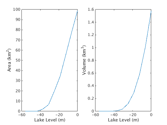
Plotting the results

We can make plots of the results using the plot function and a few associated annotation functions. To make things a bit neater, we will also use the subplot function to put our area and volume plots side-by-side in a single figure.

Remember, you can get help on all of these by typing help or doc and the function name on the command line.

We also want to make plotting optional, so let's add a logical "switch" as a parameter and use an if statement to enable or disable plotting.

% Script. Read gridded lake bathymetry data from a csv file and compute lake
% area and volume as a function of lake level.

% define parameters
file = 'data/quabbin.csv';
dx = 20; % m
dy = 20; % m
num_level = 10;
make_plot = 1; % 1 = on, 0 = off

% read in data
depth = csvread(file);

% get lake levels
level_min = -max(max(depth));
level_step = level_min/(num_level-1);
level = 0:level_step:level_min;

% create output variables
area = zeros(1, num_level);
vol = zeros(1, num_level);

% populate output variables
for i = 1:num_level

    % reduce level
    low = depth+level(i);
    wet = low>0;

    % compute area
    area(i) = sum(sum(wet))*dx*dy; % m^2

    % compute volume
    vol(i) = sum(low(wet))*dx*dy; % m^3
end

% plot, if enabled
if make_plot
    figure()

    subplot(1,2,1)
    plot(level,area/1e6);
    xlabel('Lake Level (m)');
    ylabel('Area (km^2)')

    subplot(1,2,2)
    plot(level,vol/1e9);
    xlabel('Lake Level (m)');
    ylabel('Volume (km^3)')
end

Convert script to a function

Lastly, it may be useful to convert this script to a function. The advantage is that we can hide the details behind a well-defined interface and protect our future selves from variable naming conflicts. If you plan to reuse your code, functions are simply the way to go.

Converting is surprisingly simple - we just have to add a function declaration at the start of the file. The "parameter" variables we set at the start of the script become input variables. As output variables, let's return level, area, and vol. These are the only variables we might concievable want to use for some further purpose (e.g. writing out a table).

Let's call our new function as lake_level. For MATLAB to find this name, we must also name the file lake_level.m.

The first comment following the function declaration will be displayed if someone (our future selves, most likley) types help lake_level. It is a good idea to provide a reminder of the syntax and purpose of the function.

function [level, area, vol] = lake_level(file, dx, dy, num_level, make_plot)
% function [level, area, vol] = lake_level(file, dx, dy, num_level, make_plot)
%
% Read gridded lake bathymetry data from a csv file and compute lake
% area and volume as a function of lake level.

% read in data
depth = csvread(file);

% get lake levels
level_min = -max(max(depth));
level_step = level_min/(num_level-1);
level = 0:level_step:level_min;

% create output variables
area = zeros(1, num_level);
vol = zeros(1, num_level);

% populate output variables
for i = 1:num_level

     % reduce level
     low = depth+level(i);
     wet = low>0;

     % compute area
     area(i) = sum(sum(wet))*dx*dy; % m^2

     % compute volume
     vol(i) = sum(low(wet))*dx*dy; % m^3
 end

% plot, if enabled
if make_plot
    figure()

     subplot(1,2,1)
     plot(level,area/1e6);
     xlabel('Lake Level (m)');
     ylabel('Area (km^2)')

     subplot(1,2,2)
     plot(level,vol/1e9);
     xlabel('Lake Level (m)');
     ylabel('Volume (km^3)')
 end

We can call this new function from the command line like so:

[l, a, v] = lake_level('data/quabbin.csv', 20, 20, 10, 1);