

SciVis Overview
Understanding Data Organization
(Grids, Lattices and Meshes)
These definitions provide a useful conceptual framework for discussing
data organization. Be aware that some visualization packages have their
own terminology or even creatively misuse the standard terminology.
Input data can be described by the following components:
Grid
- The set of coordinates at which data values can be located. The
points can be uniformly or non-uniformly spaced.
Topology
- The geometrical relationship between successive locations in the grid.
This is usually expressed as a dimension.
Mesh or Lattice
- A mesh (or alternatively,"lattice") is defined by its Grid and Topology.
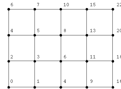
A mesh can be thought of as the domain of the data. Here is an example of a
mesh description: "uniform 2-dimensional lattice in the plane". It is shown
below. In most contexts, lattice is equivalent to Mesh, but can also mean
Mesh+Data. (This term is also used generically in Numerical Algorithms
Group Explorer to refer to data structures.)
Data
- The actual values located at the points in the grid. The "range".
Mapping Computational Space to Coordinate Space:
There are two kinds of spaces that describe your data organization,
computational space and coordinate space. Computational
space is the parameter space used to calculate or collect the data.
Coordinate space can be thought of as a mapping to "physical space".
Coordinate and computational space do not have to have the same
dimensionality, as some of the examples below will show.
Examples:
Uniform 2D Lattice in the Plane:
- Uniform distance between any coordinates along an axis, and is
the same for all axes.

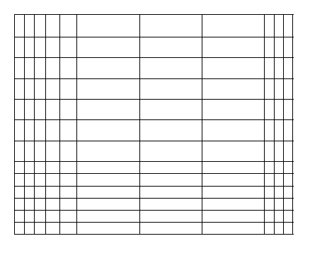
A 2D Perimeter Lattice in the Plane:
- Coordinates still lie on intersections of orthogonal grid-lines, but
there distance between any two grid-lines along an axis varies.

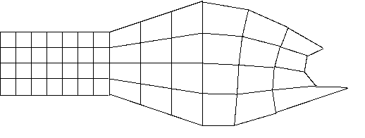
A 2D Curvilinear Lattice in the Plane:
- Also known as Curvilinear or Non-uniform. Points can exist anywhere in space.

Here are some examples that sometimes confuse people:
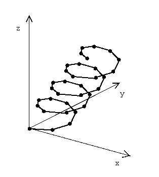
A 1D Curvilinear Lattice in 3-space:
The grid is the set of points in R^3 space, but is parameterized by
only one value, say t. Although each coordinate in the grid lives in R^3,
the next coordinate is obtained by some f(t+1). Consider this example,
a pilot flies through a storm cloud collecting water density data at
distinct time intervals. She records the density at her current location.
Her location at time t defines the points in the grid, and each successive
point in the grid can be obtained by f(t+dt), not by incrementing
x,y, and z.

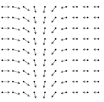
A 2D Vector field
Each point in this 2D field has a 2D vector associated with it (the data)
instead of a scalar.
